Spotting the Odd One Out: Understanding Data Anomalies using Isolation Forest

1. What's a data anomaly?

Think of a data anomaly as that unexpected guest at a party. It's data that looks different from the rest. Sometimes it's real, like a surprise celebrity appearance. Other times, it's a mistake, like someone crashing the party.

2. Why bother about these anomalies?

These unexpected guests can either make or break the party. In the same way, anomalies can twist our understanding of data, leading us to make wrong decisions. It's like judging the party vibe based on one person. By spotting these, we ensure our data tells the real story, and we can also catch sneaky issues like fraud.

3. What's the risk if we miss them?

If we ignore the party crasher, we might miss the actual vibe. Similarly, unnoticed anomalies can give us a skewed picture. But, being too picky can also mean removing some genuine, interesting data points. It's about finding the right balance.

4. So, is spotting extreme values enough?

Not really. Just like not all party crashers are loud and flashy, not all anomalies scream for attention. Some are quiet and blend in. Simply looking for extreme values might miss these subtle, yet significant, anomalies.

Outliers vs. Anomalies

An outlier is a data point that deviates significantly from other observations. It might be due to variability or perhaps an error in measurement. An anomaly is a data point that doesn't conform to the expected pattern or behavior of the dataset. All anomalies are outliers, but not all outliers are necessarily anomalies. Anomalies might represent a new, previously unseen behavior. Outlier detection methods can be used to detect anomalies, especially when we're looking for data points that are numerically distant from the rest. Some common techniques include: Statistical Methods: For example, points that fall outside of 1.5 times the interquartile range (IQR) are considered outliers. Z-Score: Data points with a z-score (a measure of how many standard deviations away a data point is from the mean) above a certain threshold can be considered outliers. Clustering Methods: Like the K-means clustering, where data points that are distant from any cluster can be considered outliers. However, there are limitations: While outlier detection can identify anomalies, it primarily focuses on extreme values. But not all anomalies are extreme values. Some might be subtle and not necessarily distant from other data points. For instance, in a time-series dataset, a slightly increased value might be an anomaly if it breaks the pattern, even if it's not an "extreme" value. While outlier detection methods can be used for anomaly detection, they're just one tool in the toolbox. Depending on the nature of the data and the kind of anomalies you're looking to detect, other methods like Isolation Forest or One-Class SVM might be more appropriate.

Enter the Isolation Forest!

Imagine a game where you try to isolate the most unique person at the party. Isolation Forest plays a similar game with data. It tries to find the quickest way to isolate these unusual data points. The faster it can do this, the more likely it is an anomaly. Another method: One-Class SVM Picture a line separating the partygoers from the empty space in the room. The One-Class SVM finds the best position for this line, ensuring maximum people are on the party side, leaving the anomalies out.

In today’s article we will focus more on Isolation Forest :

Imagine a Forest... Think of a vast forest with numerous trees. Now, instead of trees that grow leaves, imagine trees that isolate data points. In this forest, the goal of each tree is to isolate every data point by separating it from others.

The Concept of Isolation:

Random Selection: At each level of the tree, a feature from the data is randomly chosen, and then a random split value between the minimum and maximum values of that feature is selected.

Repeating the Process: The process is repeated, further subdividing the data until each data point is isolated from others, essentially making it a "leaf" in the tree.

Anomalies Are Easier to Isolate: Anomalies are "different" from other data points, right? So, they tend to get isolated much quicker than the "normal" data points. This means that the path length to isolate anomalies is typically shorter in these trees.

Aggregating Over Many Trees: The "forest" in Isolation Forest is made up of many such trees. By averaging the isolation path length over multiple trees, a score can be determined for each data point. Shorter paths generally indicate anomalies

Why It's Effective:
1) The random partitioning produces shorter paths for anomalies. So, this method is quite efficient as it doesn’t require as much time to identify anomalies as some other methods.
2) Isolation Forest works well even with high-dimensional data, where many features can make other anomaly detection methods cumbersome.
3) Unlike some methods, Isolation Forest doesn’t need a profile of "normal" data during training. It's designed to isolate anomalies, not to describe normal data.
Overall, Isolation Forest is a bit like playing a game of "spot the difference." Anomalies, being inherently different, stand out and are easier to spot (or in this case, isolate) compared to regular data points. This unique approach of focusing on isolating anomalies rather than describing the normal makes Isolation Forest a powerful tool for anomaly detection.

Lets explore a Kaggle dataset from the link https://www.kaggle.com/datasets/nelgiriyewithana/billionaires-statistics-dataset
The data set is of billionaires and we will try to detect the anomaly on the net worth and age.
import pandas as pd
from sklearn.ensemble import IsolationForest
import matplotlib.pyplot as plt

# Reading the data using 'ISO-8859-1' encoding
data = pd.read_csv('/content/billionaire data.csv', encoding='ISO-8859-1')

# Filter the data to retain only 'age' and 'finalWorth' columns and remove rows with missing values
age_finalworth_data = data[['age', 'finalWorth']].dropna()

# Apply Isolation Forest on 'age' and 'finalWorth' columns
clf_age_finalworth = IsolationForest(contamination=0.05)
age_finalworth_preds = clf_age_finalworth.fit_predict(age_finalworth_data)

# Plotting the results with improved visualization
plt.figure(figsize=(15, 7))
plt.scatter(age_finalworth_data['age'], age_finalworth_data['finalWorth'],
c=age_finalworth_preds, cmap='coolwarm', edgecolors='k', alpha=0.7)

# Highlighting anomalies with red color
anomalies = age_finalworth_data[age_finalworth_preds == -1]
plt.scatter(anomalies['age'], anomalies['finalWorth'],
c='red', label='Anomalies', edgecolors='k', s=100, zorder=5)

plt.title("Anomaly Detection using Isolation Forest on Age and Final Worth")
plt.xlabel("Age")
plt.ylabel("Final Worth (in billions)")
plt.legend()
plt.grid(True)
plt.show()

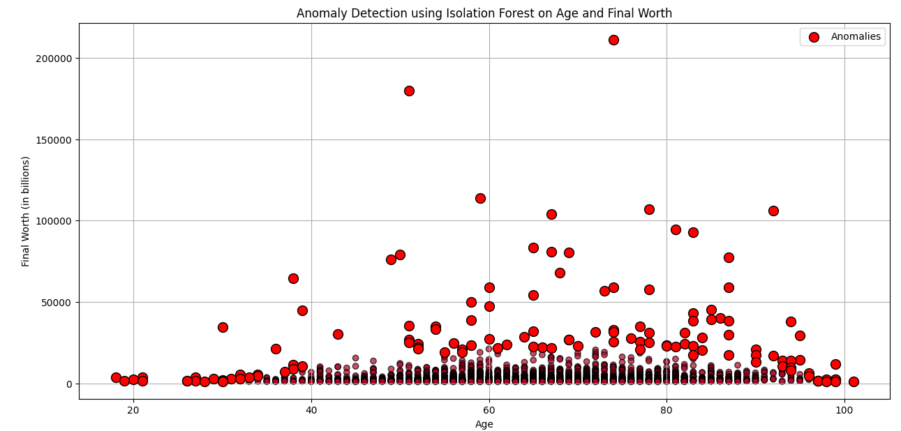
The points represent billionaires based on their "Age" (x-axis) and "Final Worth" (y-axis).
The color gradient, transitioning from blue to red, indicates the classification of each data point by the Isolation Forest model. Blue points are deemed regular, while red points are identified as anomalies.
For clearer visualization, anomalies are highlighted with a more intense red color and a larger marker size.
As seen, the Isolation Forest has detected certain billionaires, especially those with exceptionally high "Final Worth" values at varying ages, as anomalies. This provides a clearer and more intuitive visualization of the data and its anomalies.

# Create a dataframe containing only the anomalies detected by Isolation Forest on 'age' and 'finalWorth' columns
anomalies_df = age_finalworth_data[age_finalworth_preds == -1]

# Display the first few rows of the anomalies dataframe
anomalies_df.head()

# Create age bins for better visualization
bins = [0, 30, 40, 50, 60, 70, 80, 90, 100]
labels = ['0-30', '30-40', '40-50', '50-60', '60-70', '70-80', '80-90', '90-100']
anomalies_df['age_bin'] = pd.cut(anomalies_df['age'], bins=bins, labels=labels, right=False)

# Count the number of anomalies in each age bin
age_bin_counts = anomalies_df['age_bin'].value_counts().sort_index()

# Plot the bar graph
plt.figure(figsize=(12, 7))
age_bin_counts.plot(kind='bar', color='skyblue', edgecolor='black')
plt.title('Number of Anomalies in Each Age Bin')
plt.xlabel('Age Bin')
plt.ylabel('Number of Anomalies')
plt.xticks(rotation=45)
plt.grid(axis='y')
plt.show()

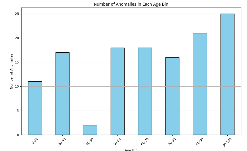
The bar graph visualizes the number of anomalies detected within each age bin.
From the graph, we can observe the distribution of anomalies across different age groups. It seems that the age groups 80-90 and 90-100 have the highest number of anomalies among the billionaires in terms of their "Final Worth".

Conclusion :

Using the information from anomaly detection, especially from methods like the Isolation Forest, can significantly enhance future model building by :

Data Cleaning and Pre-processing:
If anomalies are due to data entry errors or system faults, they can be corrected or removed to prevent models from learning from incorrect data.
For genuine anomalies that represent rare but important events (e.g., fraud detection), understanding their nature can help in feature engineering or in building specialized models.

Model Robustness:
Removing or accounting for outliers can lead to models that are more robust and less sensitive to extreme values.

Feature Engineering:
The features that contribute most to anomalies can be identified and might be especially important for the predictive task.
New features can be created, such as an "anomaly score" from the Isolation Forest, which can be used as an input to other models.

Specialized Models:
For datasets where anomalies represent critical events (like fraud, equipment failure, etc.), you can build specialized models focusing solely on these events.

Model Evaluation:
If anomalies are of particular interest, ensure that the model evaluation metric reflects the importance of correctly classifying these points. For instance, in imbalanced datasets, precision, recall, F1-score, or area under the Precision-Recall curve might be more appropriate than accuracy.

Semi-supervised Learning:
If the anomalies are labeled after detection, they can be combined with the original dataset in a semi-supervised learning approach to improve model performance.

Feedback Loop:
As new data comes in, continuously monitor for anomalies. This not only helps in keeping the data clean but also indicates if the data's nature is changing over time (concept drift), which might necessitate model retraining.

Domain Knowledge:
Sometimes, the detected anomalies might provide insights that weren't previously evident. Collaborating with domain experts can help in understanding these better and refining the model accordingly.
In principle, the knowledge from anomaly detection can guide multiple stages of the model building process, from data pre-processing to feature engineering, model selection, and evaluation. It ensures that models are built on clean, high-quality data and that they are well-tuned to the specific challenges and requirements of the task at hand.

Hope the article was a useful read. Do reach out if any one needs any further clarity on understanding Isolation forest model or need for detecting anomalies in machine learning.

References :

Yulia Gavrilova, 10th Dec 2021. Serokell.io. What Is Anomaly Detection in Machine Learning?. Accessed on 21-10-2023

Shashank Gupta, www.enjoyalgorithms.com, Introduction to Anomaly Detection in Machine Learning. Accessed on 21-10-2023

Cory Maklin, 15th Jul 2022. www.medium.com. Isolation Forest. Accessed on 21-10-2023

MLInterview, 25th September 2020. www.machinelearninginterview.com. What are Isolation Forests? How to use them for Anomaly Detection?. Accessed on 21-10-2023.